library(datasets)
library(rstan)
library(tidyverse)
library(ggplot2)
library(tidybayes)
library(brms)
theme_set(theme_minimal())Simple Mixture Models with brms and stan
Statistics
Abstract
Fitting mixture models using brms and stan, using the old faithful eruptaion data as an example.
Overview
In an attempt to learn how to fit mixture models in stan and brms, I found a blogpost on fitting a mixture model using the eruption data of old faithful. The original post implemented things in python, so I thought it would be a good exercise to try to implement it in R, using both brms and rstan.
Here’s what the dataset looks like:
Code
faithful %>%
  ggplot(aes(x = eruptions, y = waiting)) +
  geom_point()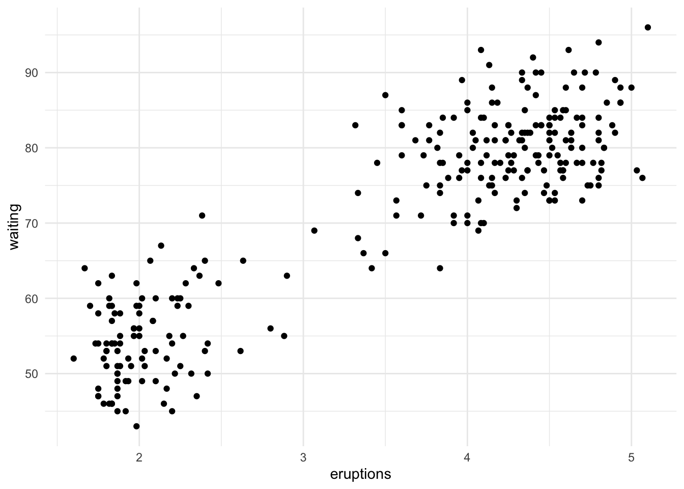
Similar to the original blog post, let’s only look at eruptions for now:
Code
faithful %>% ggplot(aes(x = eruptions)) +
  geom_dots()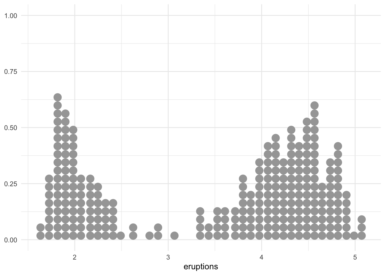
Code
# standardized version
# faithful %>% ggplot(aes(x = scale(eruptions))) +
#   geom_dots()
The data looks bimodal. We can come up with a simple mixture model:
\[ \begin{align} z_i | \theta &\sim \text{Categorical}(\theta, 1 - \theta) \\ y_i &\sim \mathcal{N}(\mu_{z_i}, \sigma_{z_i}) \\ \mu_1, \mu_2 &\sim \mathcal{N}(0, 2), \mu_1 < \mu_2 \\ \sigma_1, \sigma_2 &\sim \mathcal{N}^+(0, 2) \\ \theta &\sim \text{Beta}(5, 5) \,\,\, (*) \end{align} \]
Fit using rstan
The following stan code was directly copied from the original blog post.
stan_code <- "
data {
 int<lower = 0> N;
 vector[N] y;
}

parameters {
  ordered[2] mu;
  real<lower=0> sigma[2];
  real<lower=0, upper=1> theta;
}

model {
 sigma ~ normal(0, 2);
 mu ~ normal(0, 2);
 theta ~ beta(5, 5);
 for (n in 1:N)
   target += log_mix(theta,
                     normal_lpdf(y[n] | mu[1], sigma[1]),
                     normal_lpdf(y[n] | mu[2], sigma[2]));
}
"
Now let’s fit the model using rstan:
data <- scale(faithful$eruptions)

# create a list with the data for stan
stan_data <- list(
  N = length(data),
  y = as.numeric(data)
)

# compile the model
stan_model <- stan_model(model_code = stan_code)
Fit the model:
# fit <- sampling(stan_model,
#                 data = stan_data,
#                 chains = 4,
#                 iter = 10000,
#                 warmup = 5000,
#                 cores = 4)
#
# # save
# saveRDS(fit, file = "models/stan_faithful.rds")

fit <- readRDS("models/stan_faithful.rds")
Check the fit:
print(fit)Inference for Stan model: anon_model.
4 chains, each with iter=10000; warmup=5000; thin=1;
post-warmup draws per chain=5000, total post-warmup draws=20000.
mean se_mean sd 2.5% 25% 50% 75% 97.5% n_eff
mu[1] -1.28 0.00 0.02 -1.33 -1.30 -1.29 -1.27 -1.24 17144
mu[2] 0.69 0.00 0.03 0.63 0.67 0.69 0.71 0.75 24701
sigma[1] 0.21 0.00 0.02 0.18 0.20 0.21 0.23 0.26 17984
sigma[2] 0.38 0.00 0.02 0.34 0.37 0.38 0.40 0.43 20123
theta 0.35 0.00 0.03 0.30 0.34 0.35 0.37 0.41 22710
lp__ -252.43 0.02 1.60 -256.47 -253.24 -252.11 -251.26 -250.33 9463
Rhat
mu[1] 1
mu[2] 1
sigma[1] 1
sigma[2] 1
theta 1
lp__ 1
Samples were drawn using NUTS(diag_e) at Mon Mar 24 15:31:39 2025.
For each parameter, n_eff is a crude measure of effective sample size,
and Rhat is the potential scale reduction factor on split chains (at
convergence, Rhat=1).Let’s plot the estimated on top of existing data:
dnorm1 <- function(x) dnorm(x, mean = -1.28, sd = 0.21)
dnorm2 <- function(x) dnorm(x, mean = 0.69, sd = 0.38)
mixture <- function(x) 0.36 * dnorm(x, mean = -1.28, sd = 0.21) + (1-0.36) * dnorm(x, mean = 0.69, sd = 0.38)

data.frame(x = seq(-2, 2, 0.01)) %>%
  ggplot(aes(x)) +
  geom_dots(data = faithful, aes(x = scale(eruptions))) +
stat_function(fun = mixture, color = "maroon", linewidth = 1.2) 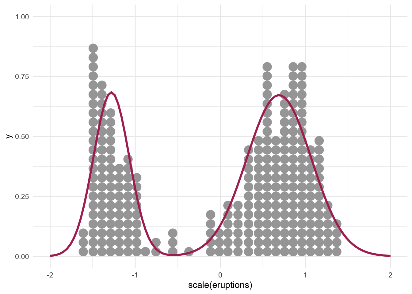
Fit using brms
Following instructions here.
mix <- brms::mixture(gaussian, gaussian)Setting order = 'mu' for mixtures of the same family.formula <- bf(eruptions ~ 1)
# get prior
get_prior(formula = formula, data = faithful, family = mix) prior class coef group resp dpar nlpar lb ub tag source
student_t(3, 0, 2.5) sigma1 0 default
student_t(3, 0, 2.5) sigma2 0 default
dirichlet(1) theta default
student_t(3, 4, 2.5) Intercept mu1 default
student_t(3, 4, 2.5) Intercept mu2 default# set prior
prior <- c(
prior(normal(0, 2), class = Intercept, dpar = mu1),
prior(normal(0, 2), class = Intercept, dpar = mu2),
# prior(beta(5, 5), class = theta), # dirichlet is the only valid prior for simplex parameters UGH
prior(normal(0, 2), class = sigma1, lb = 0), # truncated normal dist
prior(normal(0, 2), class = sigma2, lb = 0) # truncate normal dist
)Fit the model:
mixture_model <- brm(
  formula = formula,
  data = faithful,
  family = mix,
  prior = prior,
  chains = 4,
  cores = 4,
  iter = 10000,
  warmup = 5000,
  file = "models/brms_faithful"
)
Let’s see the fitted model:
summary(mixture_model) Family: mixture(gaussian, gaussian)
Links: mu1 = identity; mu2 = identity
Formula: eruptions ~ 1
Data: faithful (Number of observations: 272)
Draws: 4 chains, each with iter = 10000; warmup = 5000; thin = 1;
total post-warmup draws = 20000
Regression Coefficients:
Estimate Est.Error l-95% CI u-95% CI Rhat Bulk_ESS Tail_ESS
mu1_Intercept 2.02 0.03 1.97 2.08 1.00 16852 14234
mu2_Intercept 4.27 0.03 4.21 4.34 1.00 26116 18477
Further Distributional Parameters:
Estimate Est.Error l-95% CI u-95% CI Rhat Bulk_ESS Tail_ESS
sigma1 0.24 0.02 0.20 0.29 1.00 18701 15215
sigma2 0.44 0.03 0.39 0.49 1.00 19423 15701
theta1 0.35 0.03 0.29 0.41 1.00 20173 14603
theta2 0.65 0.03 0.59 0.71 1.00 20173 14603
Draws were sampled using sampling(NUTS). For each parameter, Bulk_ESS
and Tail_ESS are effective sample size measures, and Rhat is the potential
scale reduction factor on split chains (at convergence, Rhat = 1).pp_check(mixture_model, ndraws = 100)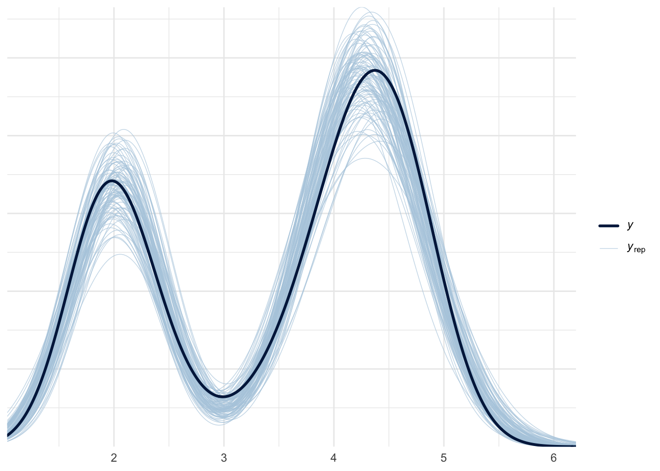
The fit seems good.
Let us draw the posterior draws:
dnorm1 <- function(x) dnorm(x, mean = 2.02, sd = 0.24)
dnorm2 <- function(x) dnorm(x, mean = 4.27, sd = 0.44)
mixture <- function(x) 0.35 * dnorm(x, mean = 2.02, sd = 0.24) + (1-0.35) * dnorm(x, mean = 4.27, sd = 0.44)

data.frame(x = seq(1, 6, 0.01)) %>%
  ggplot(aes(x)) +
  geom_dots(data = faithful, aes(x = eruptions)) +
stat_function(fun = mixture, color = "maroon", linewidth = 1.2) 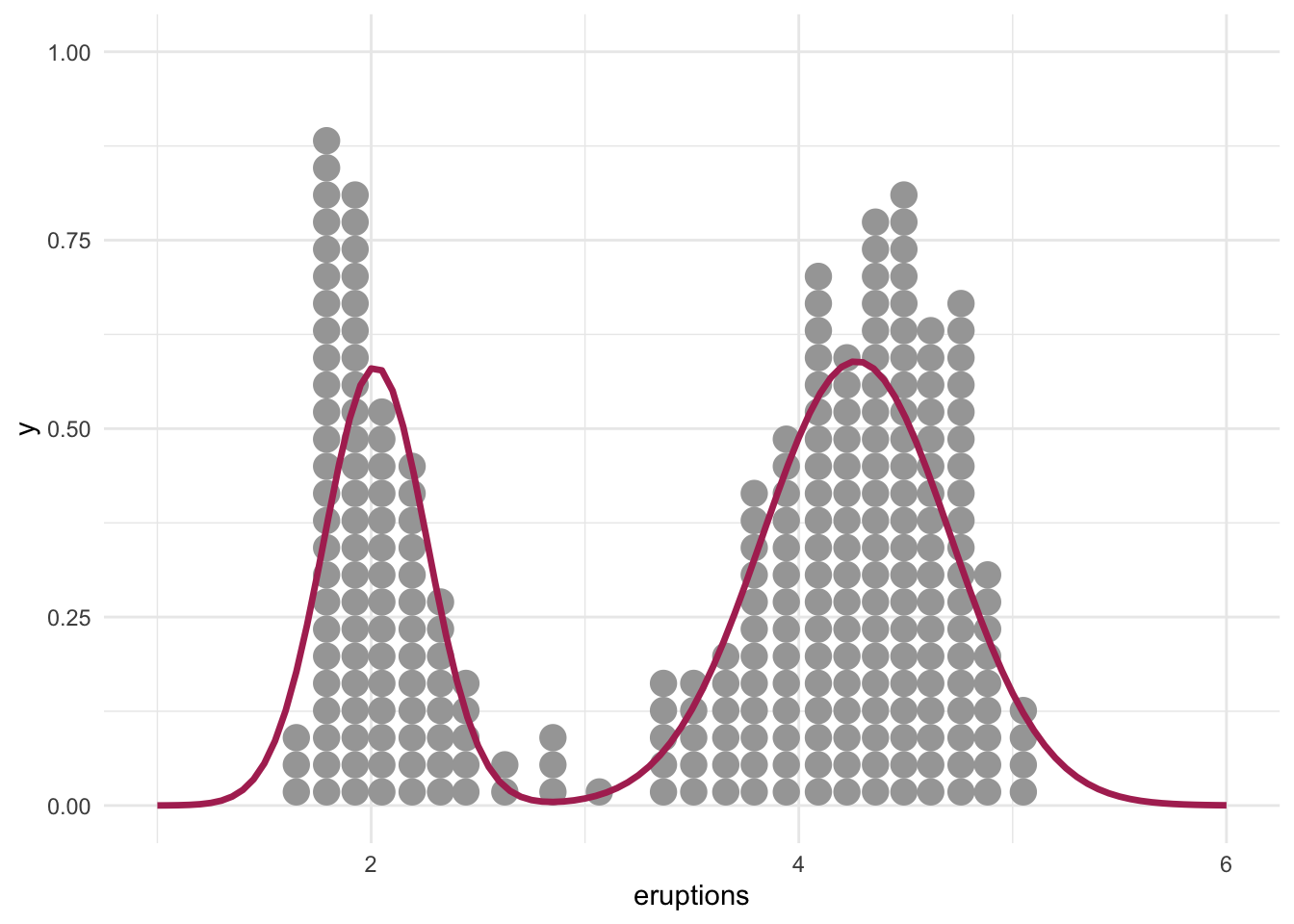
NoteWhat is the corresponding stan code?
make_stancode(formula = formula,
              data = faithful,
              family = mix,
              prior = prior)
// generated with brms 2.23.0
functions {
}
data {
int<lower=1> N; // total number of observations
vector[N] Y; // response variable
vector[2] con_theta; // prior concentration
int prior_only; // should the likelihood be ignored?
}
transformed data {
}
parameters {
real<lower=0> sigma1; // dispersion parameter
real<lower=0> sigma2; // dispersion parameter
simplex[2] theta; // mixing proportions
ordered[2] ordered_Intercept; // to identify mixtures
}
transformed parameters {
// identify mixtures via ordering of the intercepts
real Intercept_mu1 = ordered_Intercept[1];
// identify mixtures via ordering of the intercepts
real Intercept_mu2 = ordered_Intercept[2];
// mixing proportions
real<lower=0,upper=1> theta1;
real<lower=0,upper=1> theta2;
// prior contributions to the log posterior
real lprior = 0;
theta1 = theta[1];
theta2 = theta[2];
lprior += normal_lpdf(Intercept_mu1 | 0, 2);
lprior += normal_lpdf(sigma1 | 0, 2)
- 1 * normal_lccdf(0 | 0, 2);
lprior += normal_lpdf(Intercept_mu2 | 0, 2);
lprior += normal_lpdf(sigma2 | 0, 2)
- 1 * normal_lccdf(0 | 0, 2);
lprior += dirichlet_lpdf(theta | con_theta);
}
model {
// likelihood including constants
if (!prior_only) {
// initialize linear predictor term
vector[N] mu1 = rep_vector(0.0, N);
// initialize linear predictor term
vector[N] mu2 = rep_vector(0.0, N);
mu1 += Intercept_mu1;
mu2 += Intercept_mu2;
// likelihood of the mixture model
for (n in 1:N) {
array[2] real ps;
ps[1] = log(theta1) + normal_lpdf(Y[n] | mu1[n], sigma1);
ps[2] = log(theta2) + normal_lpdf(Y[n] | mu2[n], sigma2);
target += log_sum_exp(ps);
}
}
// priors including constants
target += lprior;
}
generated quantities {
// actual population-level intercept
real b_mu1_Intercept = Intercept_mu1;
// actual population-level intercept
real b_mu2_Intercept = Intercept_mu2;
}